 Dataset Prediction Model

Dataset Rating Predictor
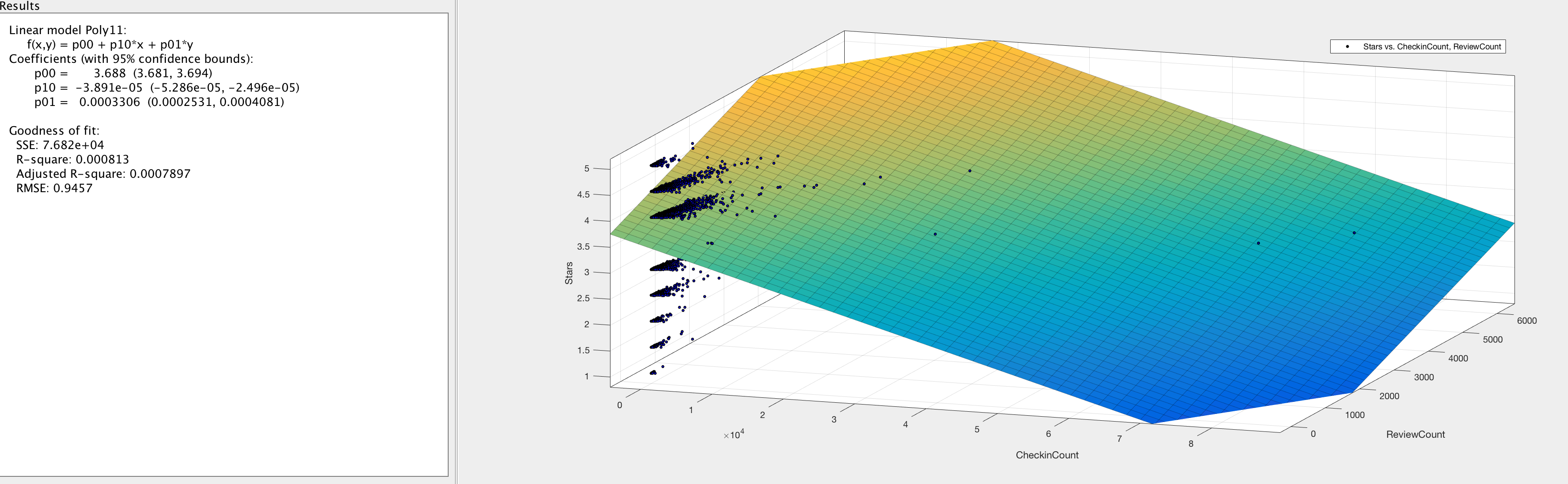
3D Surface Plot of Linear Planar Fit - Full Dataset
f(x,y) = 3.688 + -0.00003891x + 0.0003306y
where x = number of check-ins and y = number of reviews
3D Surface Plot of Linear Planar Fit - Suburban Areas
f(x,y) = 3.681 + -0.002632x + 0.00489y
where x = number of check-ins and y = number of reviews
3D Surface Plot of Linear Planar Fit - Metropolitan Areas
f(x,y) = 3.668 + -0.00002353x + 0.0002426y
where x = number of check-ins and y = number of reviews
Project Abstract
Our main focus of this project will be developing a firm understanding of the correlation that exists between the check-ins at a restaurant using Yelp and the resulting reviews given to said restaurant. We plan to use two different forms of clustering algorithms on these datasets and then analyze the results to gain insight into how each one performs and the results they grant. This analysis will be organized into a series of interactive charts and mathematical explanations for each clustering algorithm to enhance our understanding of both data visualization and grouping. From these results we hope to better understand how people eat and the behaviors they engage in following their experience and present it in a meaningful form.
The way we will conduct this project at a technical level will be through three different parts. First, we will take the JSON data from Yelp and parse it into Matlab to get relevant information for our project, upon which we will run two separate clustering algorithms. Second, we will show this data in an easily readable and interactive means on a webpage using Vis.js to represent the relevant data in charts. Finally, we will develop web based calculators to extrapolate predictions of values using the clusters that we have found to estimate restuarant outcomes.
Project Summary
We used Yelp, a service that provides customer-restaurant assessments to provide us a data set of ratings, check-ins (when a customer informs the platform that they visited a specific business), and written reviews as a way to correlate the relationships between those three variables and parse them through specific statistical algorithms, in this case, K-means clustering. We placed our results in a website for an easy, readable format. We divided our analysis into two sections, overall aggregate and selected city sub-sections. We also created a calculator in order to predict Yelp rating based on check-ins and number of written reviews. We conducted this project because Yelp is a widely used platform for assessing businesses and we wanted to see if there was a possible way to predict trends and project values such as overall ratings to help small business set specific customer goals.
Technical Walkthrough
1. Obtain Relevant Data
To download the Yelp Dataset you first have to register to join their dataset challenge on their site linked here. This allows you to choose from the businesses, check-ins, users, tips, and photos datasources, each of which is stored in JSON format. For this project we needed to obtain the businesses and check-ins files to get the amount of checkins associated with each businesses throughout the times provided, and correlate that to the business rating and review count that is specified in the businesses file.
2. Check-ins Data Format
From this sample provided by Yelp, what we can see is that the check-ins file provides a daily breakdown at hourly time intervals to show the checkins that occured throughout the week on each day and time in the entire businesses history of being on Yelp. Out of this information what we en dup being most concerned in is the encypted business id (business_id) which allows us to uniquely identify a business and the sum total of all the checkins that occur throughout the history of the business which can be pulled from the array representing the breakdown of all check-in information (checkin_info).
{
  'type': 'checkin',
  'business_id': (encrypted business id),
  'checkin_info': {
      '0-0': (number of checkins from 00:00 to 01:00 on all Sundays),
      '1-0': (number of checkins from 01:00 to 02:00 on all Sundays),
      ...
      '14-4': (number of checkins from 14:00 to 15:00 on all Thursdays),
      ...
      '23-6': (number of checkins from 23:00 to 00:00 on all Saturdays)
  }, # if there was no checkin for a hour-day block it will not be in the dict
}
3. Businesses Data Format
{
  'type': 'business',
  'business_id': (encrypted business id),
  'name': (business name),
  'neighborhoods': [(hood names)],
  'full_address': (localized address),
  'city': (city),
  'state': (state),
  'latitude': latitude,
  'longitude': longitude,
  'stars': (star rating, rounded to half-stars),
  'review_count': review count,
  'categories': [(localized category names)]
  'open': True / False (corresponds to closed, not business hours),
  'hours': {
      (day_of_week): {
          'open': (HH:MM),
          'close': (HH:MM)
      },
      ...
  },
  'attributes': {
      (attribute_name): (attribute_value),
      ...
  },
}
From this sample provided by Yelp, what we can see is that the businesses file provides basic information like the type of business its name, neighborhood, address, city, state, etc. But for our project the main concern was the encrypted business id (business_id), the city (city), the business ratings (stars), and the amount of reviews provided for the restaurant (review_count). From this information we can get identify a business in a specific city that we have chosen to represent either a large metropolitan area or smaller suburban township, and map that to the number of check-ins that have been logged, as well as provide the corresponding rating and review count totals.
4. Parsing the Data (Conceptual)
Conceptually what we want to do is first parse through all of the check-in data provided by Yelp, and for each business get the total amount of check-ins that occur throughout the entire history of the business, and then finally map them to the business id in the object format {business_id: total_checkins}. From there we can parse through the businesses data and at each value map the business id provided to the newly parsed check-ins file to get total check-ins and create an object for each business in the format {business_id: [rating, review_count, total_checkins]}. This process can also be modified to only include certain cities by only choosing to log businesses that have a matching 'city' parameter in their object definition. Now that we have a JSON object that represents all important data for us it has to be brought into a useable MATLAB format to run K-means clustering algorithms on for analysis. This is achieved using the JSONlab plugin for MATLAB that converts the JSON sting into a structure format representing all the data. Finally this structure has to be parsed one at a time and account for null data entries (when there are no recorded check-ins) and then create a usable a matrix format of just relevant data.
5. Parsing the Check-ins
/*Create a usable data format of {businessid: total checkins}*/
var fs = require('fs');

var checkIns = {};
var checkInRaw = fs.readFileSync('../data/yelp_academic_dataset_checkin.json', 'utf8').toString().split("\n");
for (var j = 0; j < checkInRaw.length -1; j++){
  checkInRaw[j] = JSON.parse(checkInRaw[j]);
  var totalCheckIns = 0;
  var keys = Object.keys(checkInRaw[j].checkin_info);
  var businessKey = checkInRaw[j].business_id;
  for(var i = 0; i < keys.length; i++){
    totalCheckIns += checkInRaw[j].checkin_info[keys[i]];
  }
  checkIns[businessKey] = totalCheckIns;
}

fs.writeFile('../data/yelp_checkins.json', JSON.stringify(checkIns, null, 2), function(err){
  if(err){
    return console.log(err);
  }
});
6. Parsing the Businesses
/*Create a usable data format of {businessid: [rating, review count, checkin count]}*/
var fs = require('fs');

var businesses = {};
var businessesRaw = fs.readFileSync('../data/yelp_academic_dataset_business.json', 'utf8').toString().split("\n");
var checkins = JSON.parse(fs.readFileSync('../data/yelp_checkins.json', 'utf8'));
for (var j = 0; j < businessesRaw.length - 1; j++){
  businessesRaw[j] = JSON.parse(businessesRaw[j]);
  businesses[businessesRaw[j].business_id] = [businessesRaw[j].stars, businessesRaw[j].review_count, checkins[businessesRaw[j].business_id]];
}

fs.writeFile('../data/yelp_businesses_all.json', JSON.stringify(businesses, null, 2), function(err){
  if(err){
    return console.log(err);
  }
});
Data split by cities script here.
7. Parsing the JSON
function return_mat = RemoveNulls(input)
  result_cells = struct2cell(input(1,1));
  return_mat = [];
  for i=1:length(result_cells)
    try
      cell = cell2mat(result_cells(i));
    catch
      result_cells{i,1}{3} = 0;
      cell = cell2mat(result_cells{i});
    end
    return_mat = [return_mat; cell];
  end
end
8. Target Clustering for Population Density Comparison
One thing that we wanted to explore was how different population densities would affect the results in our clustering. To analyze this futher we sifted through our data to see large concentrations of businesses in certain cities that we could define as being large metropolitan areas, and areas a lower but still large enough data space to analyze as what we can define as a suburban area (~50-100 businesses).
9. Cities Chosen for Target Clustering
Large Cities/Metropolitan Areas
Las Vegas, Nevada
- Population: 603,488
- Number of Businesses: 19,328
Phoenix, Arizona
- Population: 1,513,000
- Number of Businesses: 11,852
Charlotte, North Carolina
- Population: 789,862
- Number of Businesses: 5,695
Small Cities/Suburban Areas
Carnegie, Pennsylvania
- Population: 7,947
- Number of Businesses: 62
San Tan Valley, Arizona
- Population: 81,231
- Number of Businesses: 100
Belmont, North Carolina
- Population: 10,412
- Number of Businesses: 83
10. Plotting Our Data
Once we aggregated all of our data we ran the K-means clustering algorithm in MATLAB with our parsed data to determine any cluster trends across specific permutations of paired data sets. We determined this through what seemed to be most likely to give an obvious trend through observations of the paired sets. The data is displayed as follows for the overall and sub-sectioned aggregates.
Full Dataset K-Means
K-Means Plot of the ratings of each of the business versus the number of reviews for the entire dataset.
1st cluster - 3.8602, 968.0172, K = 2
2nd cluster - 3.6937 27.9724, K = 23
For the first cluster of data there seems to be a slight increase in the average rating, given a large amount of user reviews. This seems to signify that a higher volume of user ratings may typically imply popularity, which could influence users to give higher ratings. However it is possible that this change could just be due to random variation, but given the large sample size of the entire data set, it can be safe to say that this slight change is relatively accurate without completely resampling the data set.
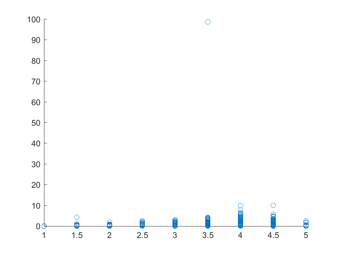
K-Means Plot of the ratings of each of the business versus the number of checkins for the entire dataset.
1st cluster - 3.6618, 13,304, K = 2
2nd cluster - 3.6949 98.7103, K = 28
For the second cluster of data we found that rating and the number of Check-ins have no significant impact on each other. Both data clusters gave a similar rating average despite the second cluster having a significant amount of check-ins per business.It can definately be said that one can conclude nothing from the clustering due to the apparent lack of variation among the data fields.
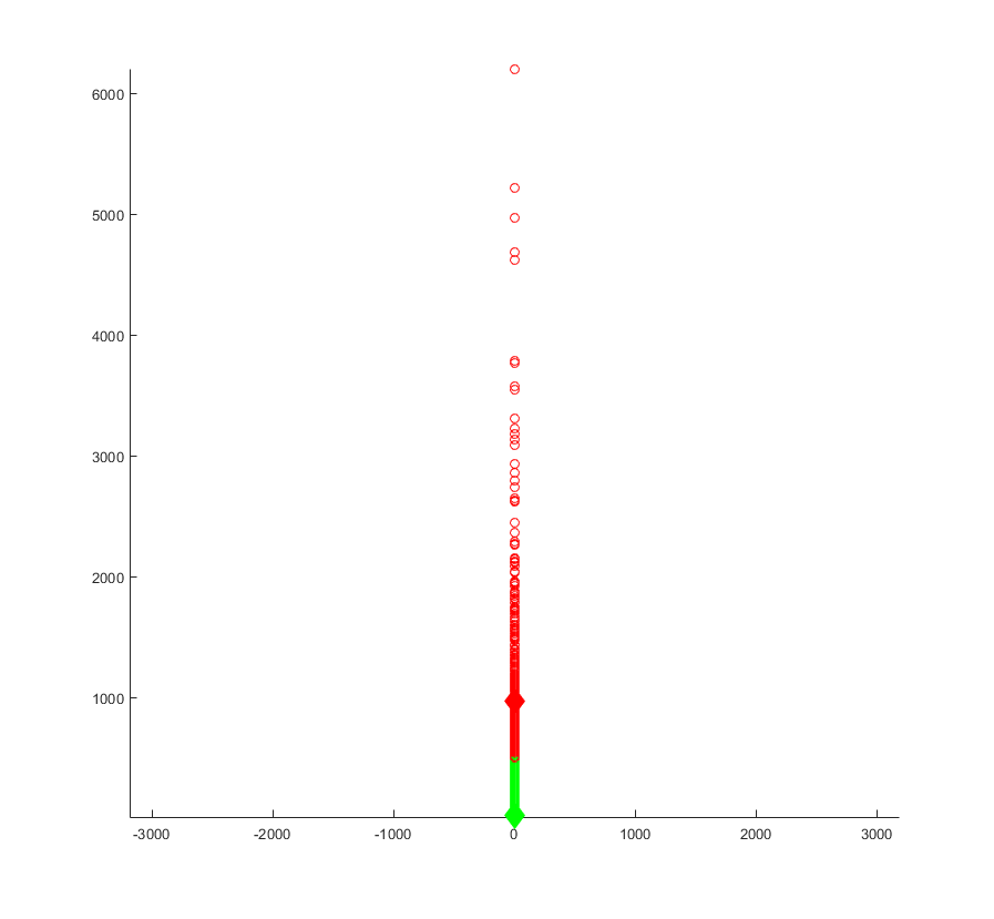
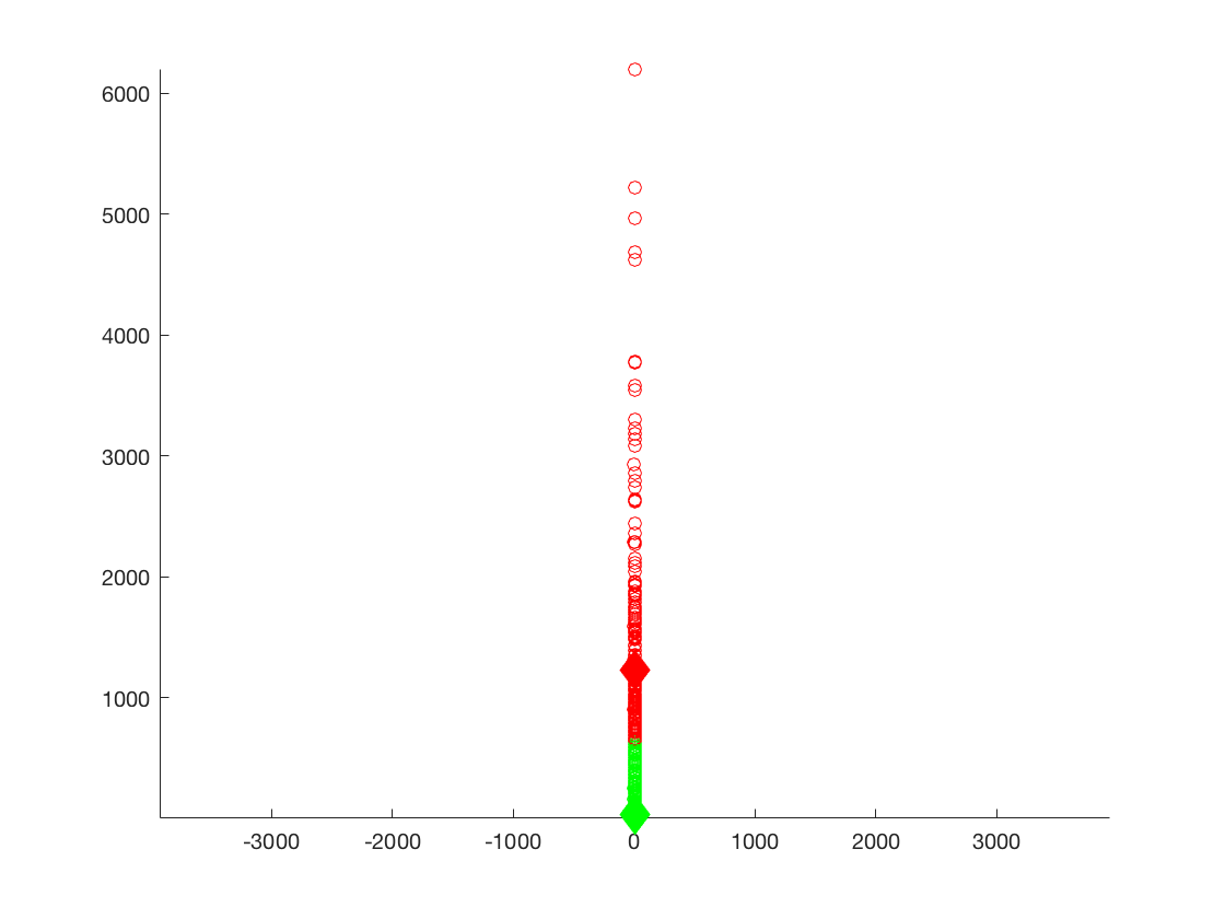
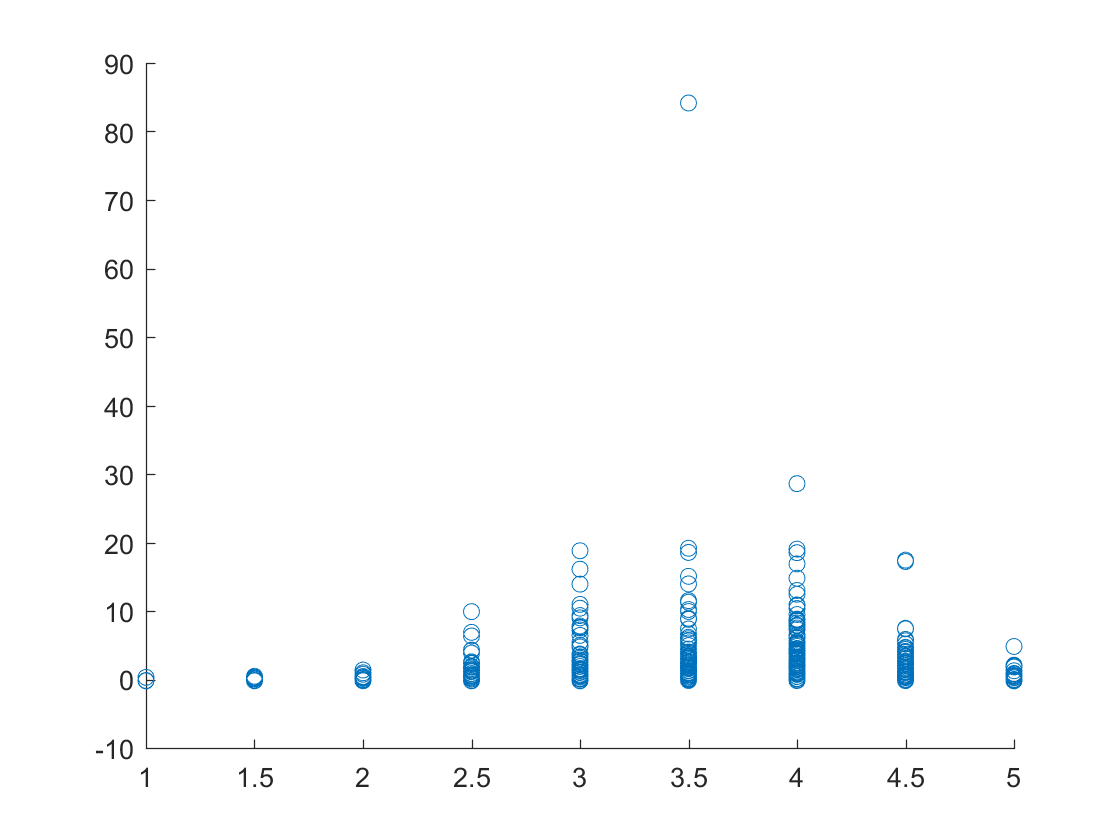
K-Means Plot of the number of reviews versus the number of checkins for the entire dataset.
1st cluster - 1,940.7, 13,303, K = 2
2nd cluster - 32.8421, 98.7113, K = 30
For the third data set it can be seen from the first cluster that a large amount of reviews result in significantly large amounts of check-ins and from the second cluster a small amount of reviews result in smaller amounts of check ins. This can be easily explained as typically popular business are promoted to incentivize their customers to check-in for some added benefit. Another aspect that this clustering uncovers is the disparity between popular and unpopular businesses, that the difference is vast enough to be extremely polarizing.
Suburban Areas K-Means
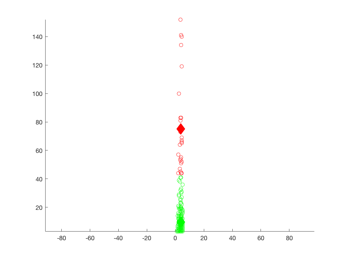
K-Means Plot of the ratings of each of the business versus the number of reviews for the suburban areas.
1st cluster - 3.7222, 75.1111, K = 2
2nd cluster - 3.6789, 9.5963, K = 5
For the first clusters of data it can be seen that the averages are much lower compared to the previous two data sets. This is probably indicative that smaller populations have smaller numbers of active users for yelp. The ratings for each cluster suggest that there is a higher concentration of similar ratings in smaller cities. This could be because smaller populations propagate opinions faster, leading to a growing similarity between user ratings of businesses.

K-Means Plot of the ratings of each of the business versus the number of checkins for the suburban areas.
1st cluster - 3.6875, 15.6964, K = 2
2nd cluster - 3.6429, 184.9524, K = 8
For the second clusters of data, like all of the other respective cluster sets, the values in each cluster show little variation and are therefore no particular conclusions can be drawn from the specific set of clusters. But it can be seen from the similarity that Yelp activity is proportionally the same for users as concluded in the large cities cluster set.
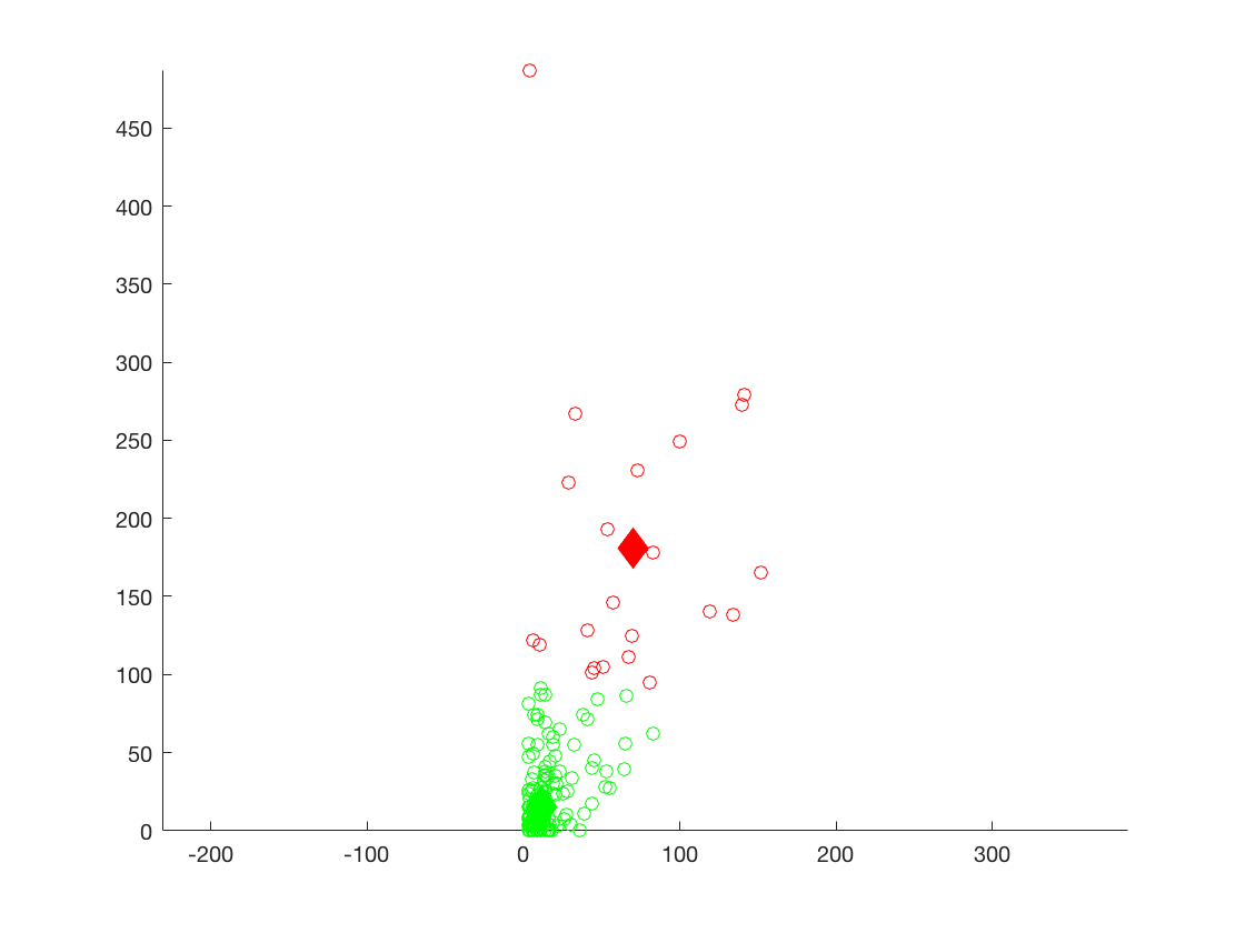
K-Means Plot of the number of reviews versus the number of checkins for the suburban areas.
1st cluster - 69.6818, 180.8636, K = 2
2nd cluster - 11.6009, 15.3408, K = 7
For the third clusters of data, again, population seems to be affecting values of each cluster, the averages for the smaller data set is significantly smaller indicating that in smaller cities there are less users and possibly less restaurants available for review.
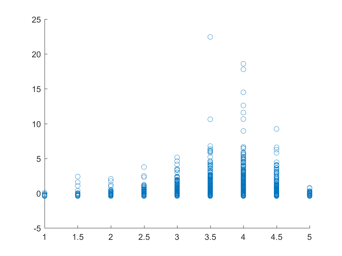
Suburban Areas Z-Scored Data

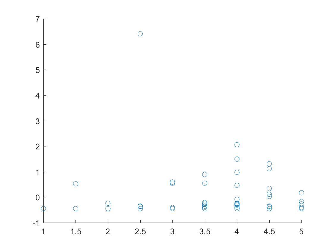
Plot of the ratings of each of the business versus the number of checkins for Belmont, North Carolina.

Plot of the ratings of each of the business versus the number of reviews for Belmont, North Carolina.
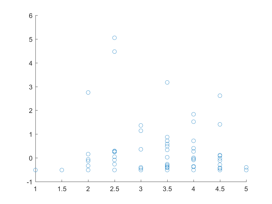
Plot of the ratings of each of the business versus the number of checkins for Carnegie, Pennsylvania.

Plot of the ratings of each of the business versus the number of reviews for Carnegie, Pennsylvania.
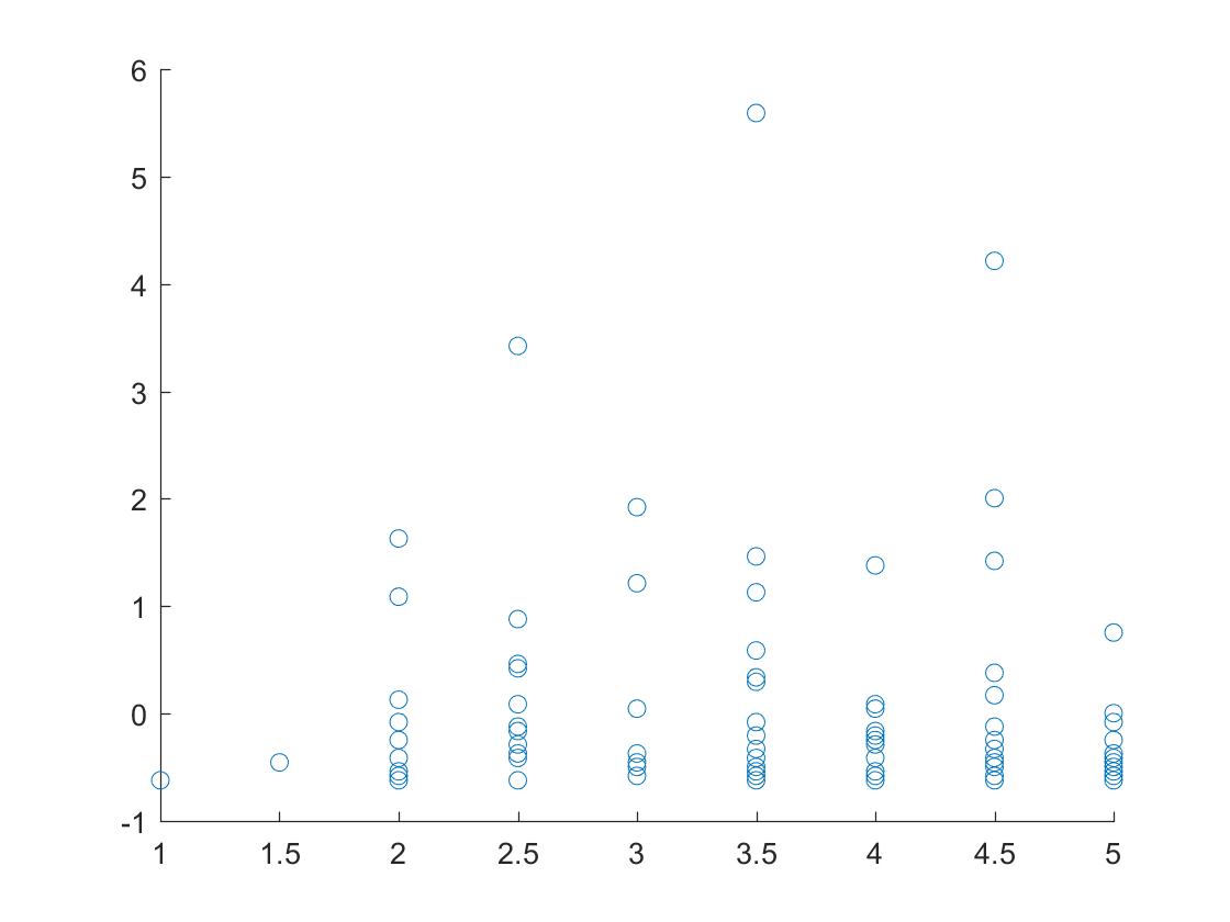
Plot of the ratings of each of the business versus the number of checkins for San Tan Valley, Arizona.
Plot of the ratings of each of the business versus the number of reviews for San Tan Valley, Arizona.
Metropolitan Areas K-Means
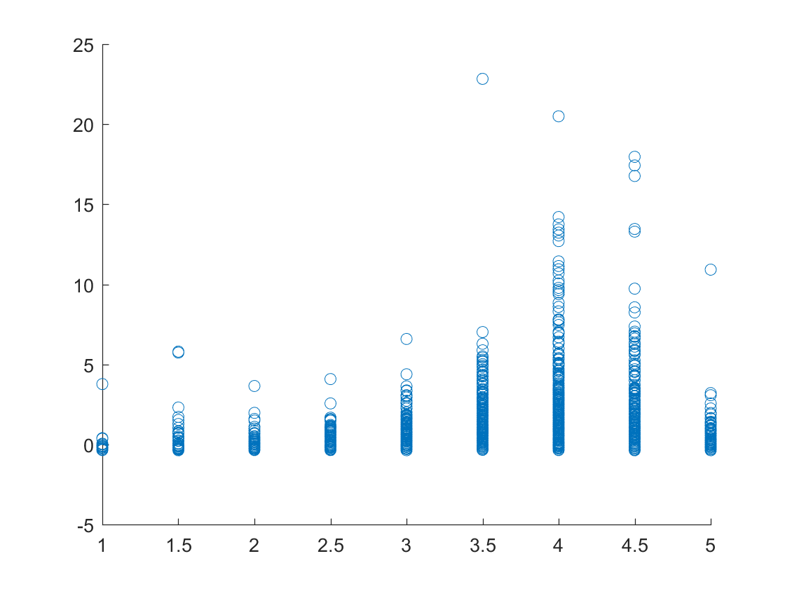
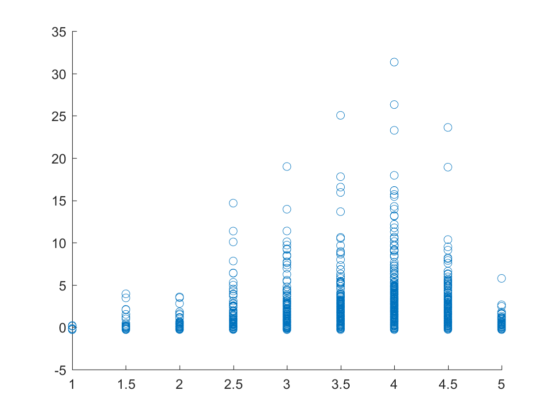
K-Means Plot of the ratings of each of the business versus the number of reviews for the metropolitan areas.
1st cluster - 3.8218, 1,224.98, K = 2
2nd cluster - 3.6737, 35.3996, K = 29
For the first clusters of data it is apparent that it resembles the values of the overall data set with slight variation, the values for each cluster seem to be slightly lower, especially the rating values. Each cluster seems to have a higher value of number of reviews, this is expected due to the large populations found in metropolitan cities.
K-Means Plot of the ratings of each of the business versus the number of checkins for the metropolitan areas.
1st cluster - 3.6786, 14,568, K = 2
2nd cluster - 3.6750, 134.8531, K = 17
For the second clusters of data we found that the values are once again, similar to its overall counterpart. Ratings compared to number of check-ins seem to be similar additionally with the small cities data set. This seems to suggest that population numbers don’t necessarily affect yelp activity for users.
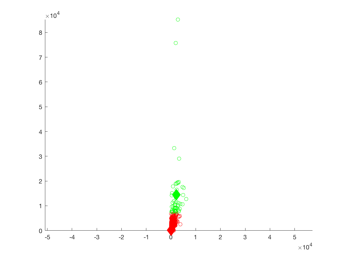
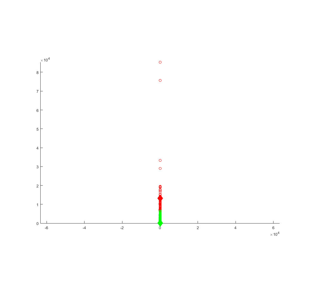
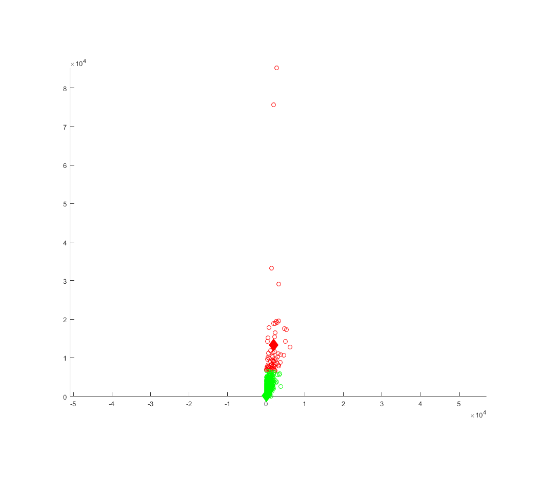
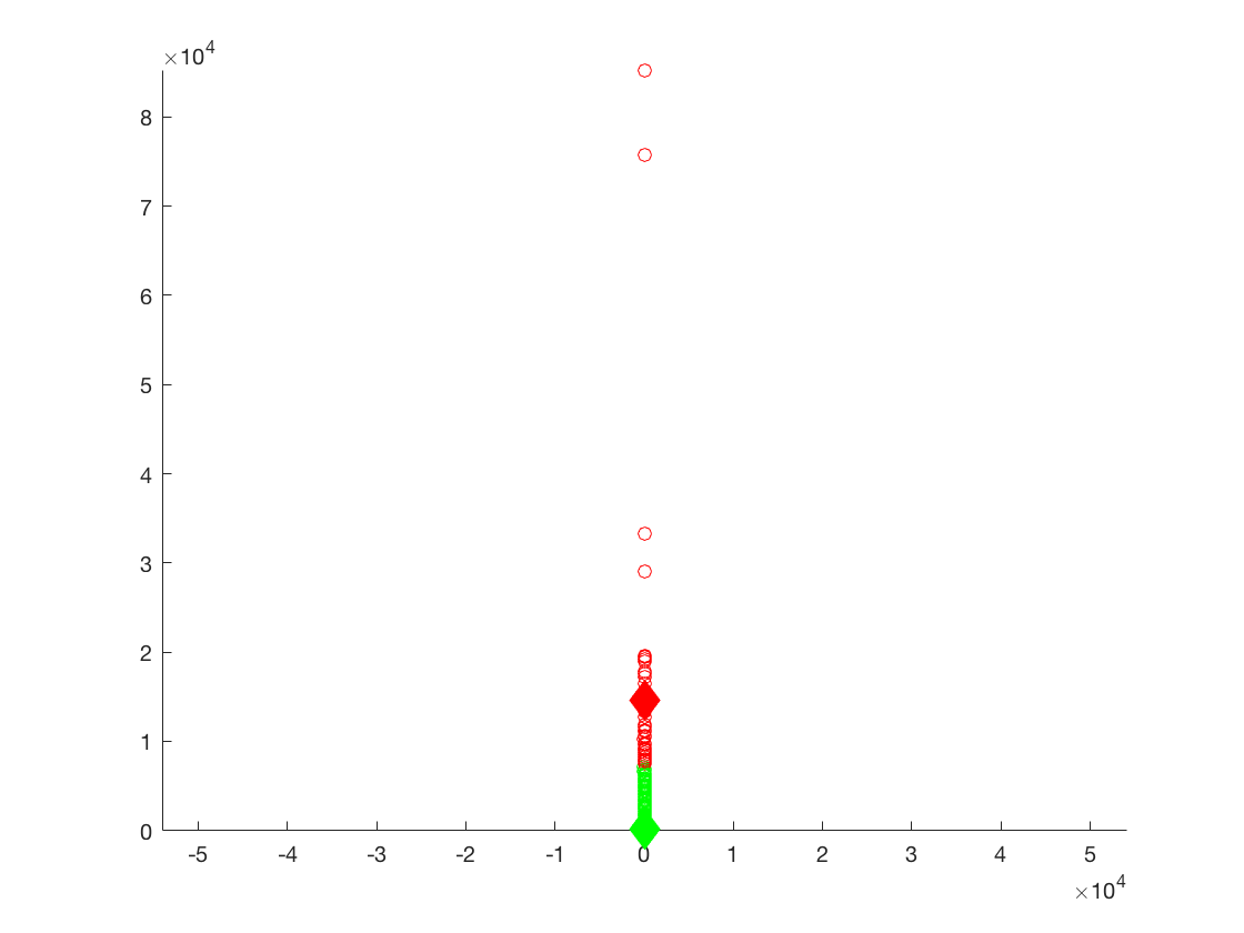
K-Means Plot of the number of reviews versus the number of checkins for the metropolitan areas.
1st cluster - 42.8709, 134.6624, K = 2
2nd cluster - 2117.4, 14,438, K = 17
For the third clusters of data it can be seen once again that due to a higher population found in cities, that all values in each cluster are higher than the overall data set. The same trends noticed in the overall set are apparent in this set of clusters as well.
Metropolitan Areas Z-Scored Data

Plot of the ratings of each of the business versus the number of checkins for Charlotte, North Carolina.
Plot of the ratings of each of the business versus the number of reviews for Charlotte, North Carolina.
Plot of the ratings of each of the business versus the number of checkins for Phoenix, Arizona.
Plot of the ratings of each of the business versus the number of reviews for Phoenix, Arizona.
Plot of the ratings of each of the business versus the number of checkins for Las Vegas, Nevada.
Plot of the ratings of each of the business versus the number of reviews for Las Vegas, Nevada.
Curve Fitting on Dataset
Fitting a linear plane equation to the entire dataset to find a rating based on the input of review count and checkin count. This process was replicated for both Suburban and Metropolitan areas as well to get unique equations for each.
Project Conclusion
If we were to improve this project we would aggregate more data from other cities, the larger the sample, the more indicative observed trends would be in terms of all the users of Yelp. We would also utilize different clustering algorithms such as spectral clustering and mixture gaussian distributions in order to find out other possible patterns and conclusions to be drawn from the data.
From the analysis of all data sets we learned that population is a factor in the trends of ratings, check-ins, and reviews. However, it can also be seen that the changes are also very slight, showing that it is not as important as we previously thought. Overall, there is a trend that large amounts of user reviews indicate higher average ratings of restaurants as well as for check ins. Activity of users towards a particular business is a positive trend: the more users interact with a business’ Yelp page, the more likely the business is to receive higher values in check-ins reviews and ratings.
Project Postmortem
Throughout our project we experienced several problems in conducting our algorithms. Our first problem was that though the Yelp data set was supposed to be in a JSON format, the actual contents of the data set were not formatted correctly as instead of being one large contiguous object, it was line separated JavaScript Objects, placing extra work on us to parse through the data before it could even be brought into a readable MATLAB format. Our solution to fix this problem was to use three separate parsing algorithms, one for parsing through associated business id’s and check-ins along with the check-in data, another for parsing through associated business id’s and reviews and ratings, and another for associating the business id’s with all of the other variables. This was an extremely difficult challenge for us to overcome, as the data was additionally formatted horribly. For example, Las Vegas had eight different identifiers(Las Vegas, las vegas, las Vegas, NV, etc.) which made it difficult to condense into one identifier given the other set of difficulties we had in the JSON file. Our second problem that we encountered was us dealing with buggy MATLAB builds that made our code not work despite it being syntactically correct. We had to restart MATLAB many times to resolve this at each iteration of our process. We found that our original data sub-sections did not display any significant obvious trends, so we decided to combine all of categories to find overall patterns in the biggest possible scope and to compare them with our sub-sectioned data. This meant combining all city data into one large aggregate. We also had issues with finding a good geometric fit for our data plots, we resolved this by using the curve-fitting toolbox from MATLAB to create a regression plane from the plot.
Created by Shivam Sharma, Kenny Wibowo, Varun Sujit, and Joseph Thomas.
All data and code used can be found in our public repository here.